OWS Styling HOW-TO Guide: Transparency
Table of Contents
Transparency in Datacube OWS
Transparency is a powerful tool for web maps. As well as basic recurring use cases like masking out missing or invalid data, partial transparency can also be used to crafting novel ways of delivering additional information.
Datacube OWS has four 1 different ways of achieving transparency.
We’ve already seen how to use transparency in colour-ramp styles in the last chapter, and in colour-map styles in this one. Both used an entry called “alpha”. The context differed, but the semantics were the same: a float between 0.0 (fully transparent) and 1.0 (fully opaque).
The remaining two approaches to transparency are the subject of this chapter.
- 1
Actually five, but one is beyond the scope of this HOWTO.
Masking
Masking can be achieved with all style types using the pq_mask element. PQ stands for
“pixel quality” and is an historical relic.
No partial transparency is possible with masking alone - masking can only make pixels fully transparent. However, the alpha channel from the underlying style (component, ramp or map) is used when applying the mask, so you can combine masking with the alpha-based transparency method appropriate to the style.
Masking (like colour map styles) requires a discrete (bitflag or enumeration) measurement band. It can still be used with continuous band component or ramp styles however, if the one ODC product contains both discrete and continuous measurement bands, or if the masking bands are drawn from separate ODC products.
Example Data for Masking
For the examples here I am masking with the Collection 3 WOFS example from the previous chapter, with continuous data from the Collection 3 Fractional Cover product:
import xarray as xr
from datacube import Datacube
dc = Datacube()

wofs_data = dc.load(
    product='ga_ls_wo_3',
    measurements=['water'],
    latitude=(-15.9098, -15.0496),
    longitude=(128.0882, 129.2171),
    time=('2020-12-08T10:00:00', '2020-12-09T09:59:59'),
    output_crs="EPSG:3577",
    resolution=(-120,120),
    group_by="solar_day"
)

fc_data = dc.load(
    product='ga_ls_fc_3',
    measurements=['bs', 'pv', 'npv'],
    latitude=(-15.9098, -15.0496),
    longitude=(128.0882, 129.2171),
    time=('2020-12-08T10:00:00', '2020-12-09T09:59:59'),
    output_crs="EPSG:3577",
    resolution=(-120,120),
    group_by="solar_day"
)

# Time coordinates come back slightly differently from the two products, so we need
# to align them before we combine.

wofs_data.coords["time"] = fc_data.coords["time"]
combined_data = xr.combine_by_coords(
        [fc_data, wofs_data],
        join="exact")
Example: No Masking
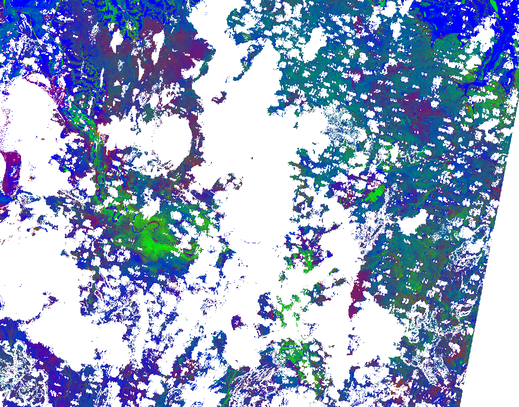
The main fractional cover view is component based view with “bare soil (bs)” band mapped to red, the “photosynthetic vegetation (pv)” band mapped to green and the “non-photosynthetic vegetation (npv)” band mapped to blue.
unmasked_fc_cfg =  {
    "components": {
        "red": {"bs": 1.0},
        "green": {"pv": 1.0},
        "blue": {"npv": 1.0}
    },
    "scale_range": [0.0, 100.0],
}
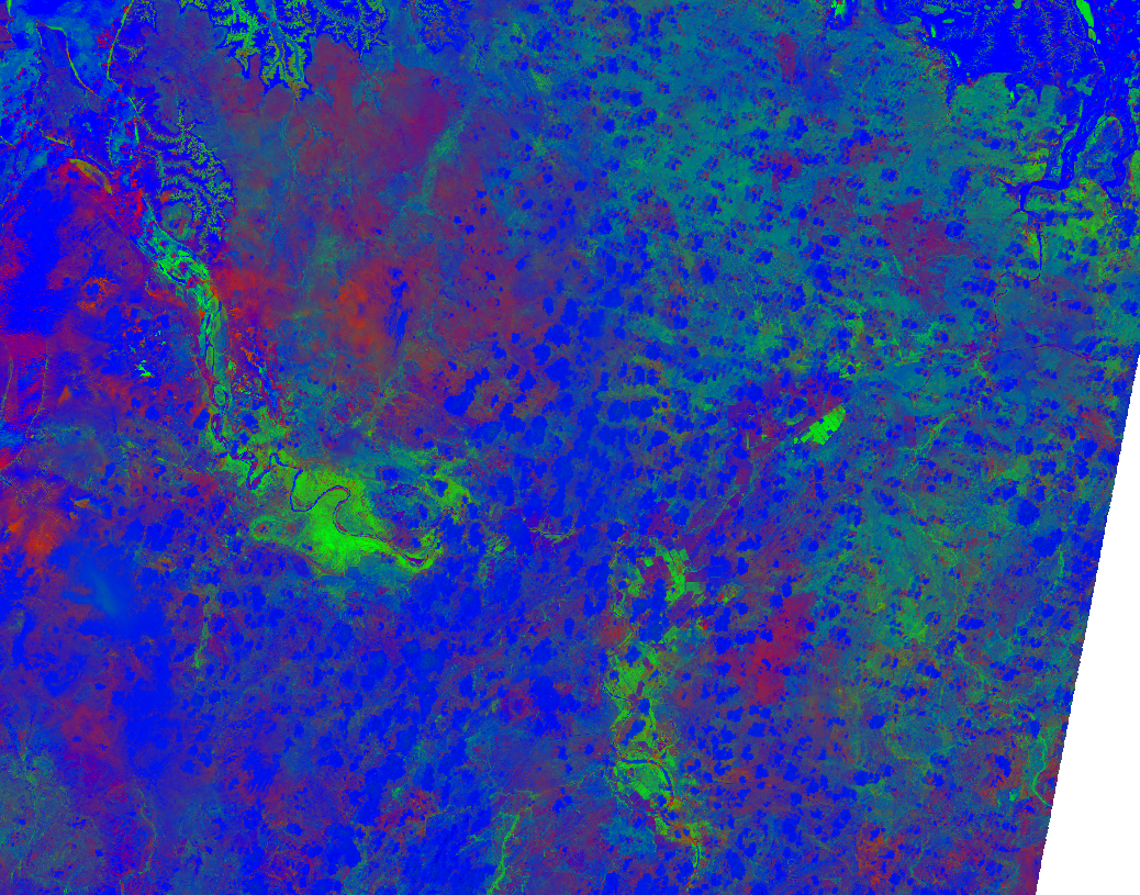
As you can clearly see from comparing this image to the colour map examples in the last chapter, areas of cloud and water give false positives as npv.
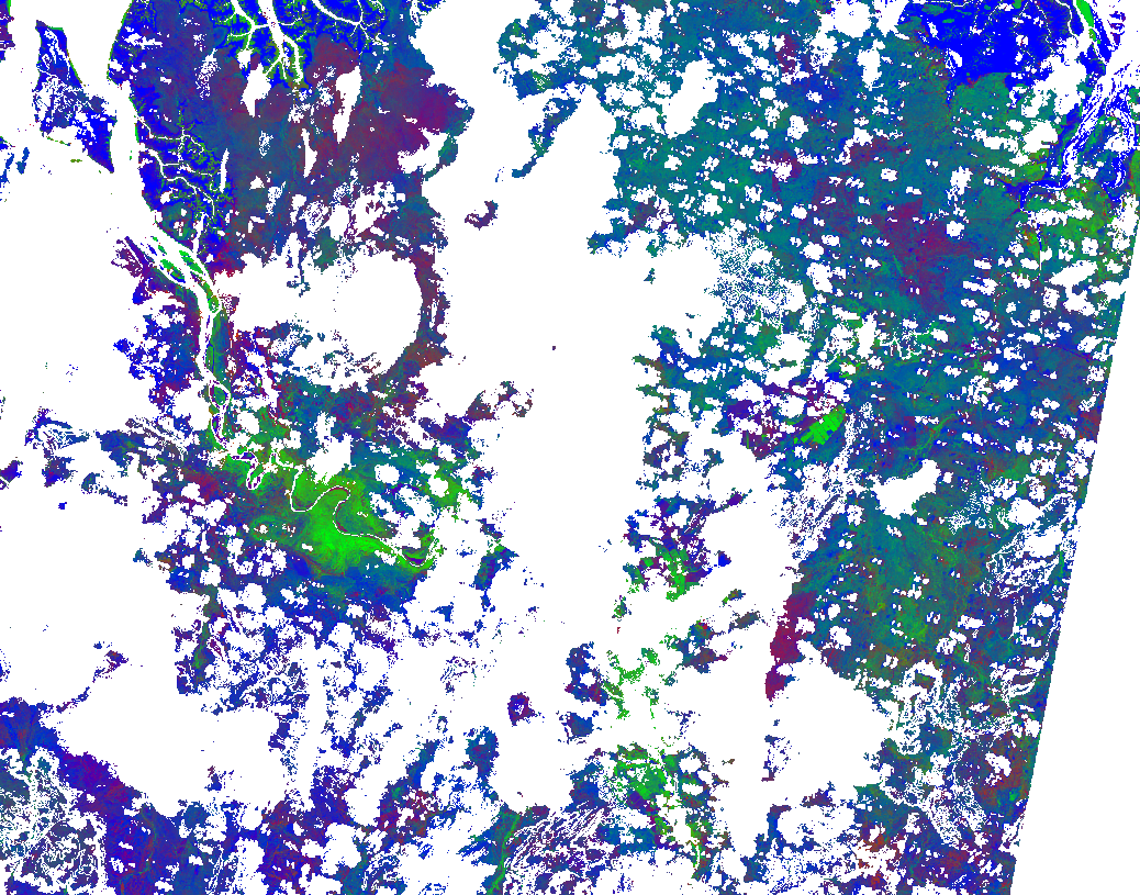
Example: Masking out invalid pixels
Masking uses a similar syntax to colour maps flags rules. You specify the values you want to keep in the image - pixels that fail any of the pq_mask rules will be transparent.
masked_fc_cfg =  {
    "components": {
        "red": {"bs": 1.0},
        "green": {"pv": 1.0},
        "blue": {"npv": 1.0}
    },
    "scale_range": [0.0, 100.0],
    "pq_masks": [
        # Pixels must match all flags to remain visible.
        {
            "band": "water",
            "flags": {
                "nodata": False,
                "noncontiguous": False,
                "terrain_shadow": False,
                "low_solar_angle": False,
                "high_slope": False,
                "cloud_shadow": False,
                "cloud": False,
                "water_observed": False,
            }
        }
    ]
}
Example: Enumeration masking
For non-bitflag discrete measurement bands, it is necessary to specify the exact values to mask on, this
can be done using enum masking rules:
enum_masked_fc_cfg =  {
    "components": {
        "red": {"bs": 1.0},
        "green": {"pv": 1.0},
        "blue": {"npv": 1.0}
    },
    "scale_range": [0.0, 100.0],
    "pq_masks": [
        {
            "band": "water",
            "enum": 1, # 1 = nodata
        }
    ]
}
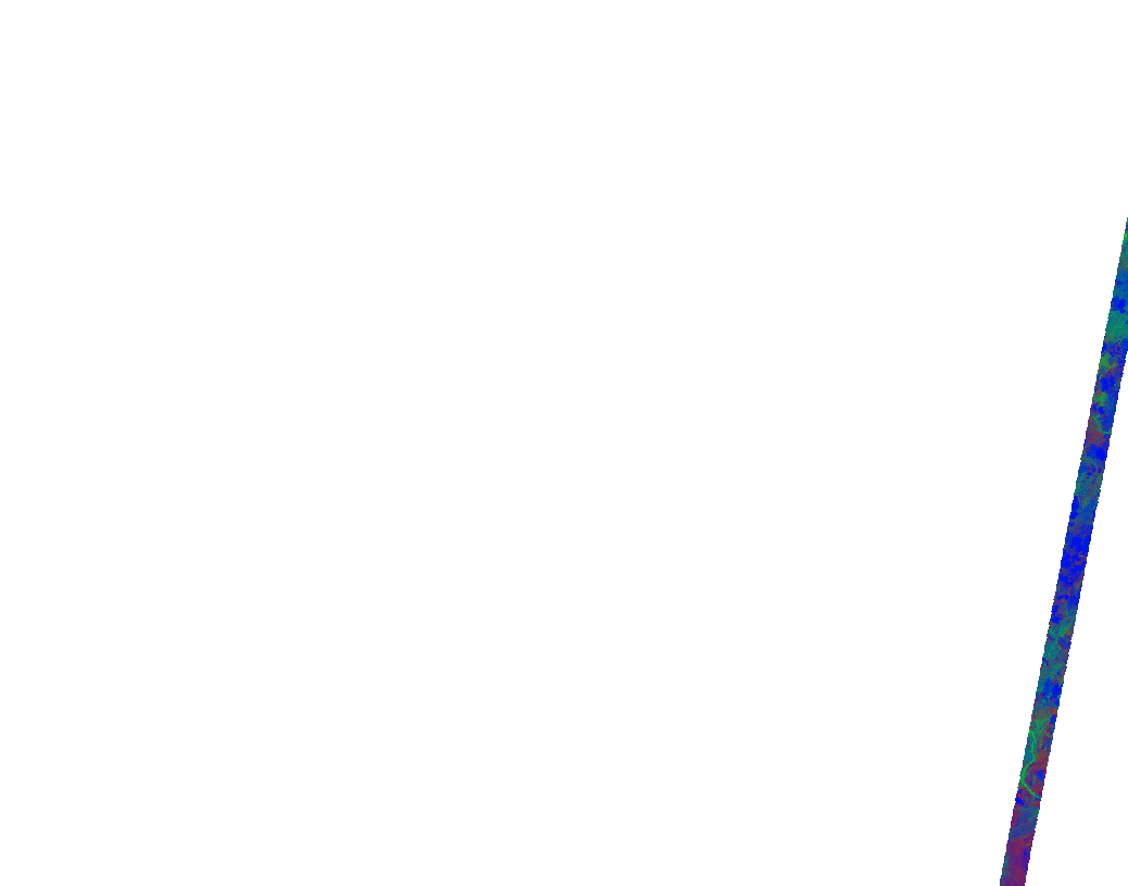
What happened here? Remember pq_masking rules specify the values to keep, so setting enum to 1 means that we only keep pixels which are marked nodata in WOFS - everything else becomes transparent.
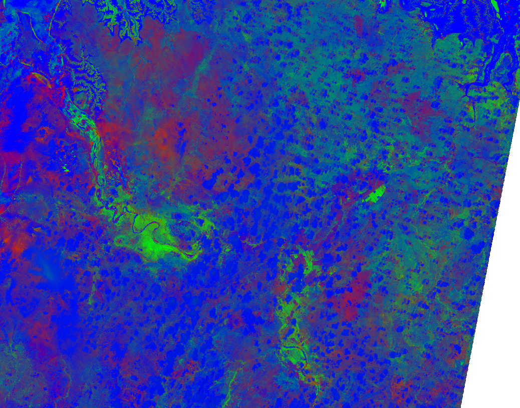
Example: Inverted enum mask
Luckily there’s an easy fix - we can add “invert” to the rule to reverse the logic - keep pixels that DON’T match the rule and make pixels that do transparent:
inverted_masked_fc_cfg =  {
    "components": {
        "red": {"bs": 1.0},
        "green": {"pv": 1.0},
        "blue": {"npv": 1.0}
    },
    "scale_range": [0.0, 100.0],
    "pq_masks": [
        {
            "band": "water",
            "enum": 1,
            "invert": True,
        }
    ]
}
Example: Complex logic
Finally we look at a more complex example:
complex_masked_fc_cfg = {
    "components": {
        "red": {"bs": 1.0},
        "green": {"pv": 1.0},
        "blue": {"npv": 1.0}
    },
    "scale_range": [0.0, 100.0],
    "pq_masks": [
        {
            # Mask out nodata pixels.
            "band": "water",
            "enum": 1,
            "invert": True,
        },
        {
            # Mask out pixels with low_solar_angle, high_slope
            #      or cloud shadow.
            "band": "water",
            "flags": {
                "low_solar_angle": False,
                "high_slope": False,
                "cloud_shadow": False,
            }
        },
        {
            # Mask out pixels with cloud AND no water observed
            "band": "water",
            "flags": {
                "cloud": True,
                "water_observed": False,
            },
            "invert": True,
        },
    ]
}
This is not a particularly useful visualisation, but it hopefully demonstrates how everything fits together when building up mask logic.
Alpha Masking in Component Styles
We have seen how to do simple (non-alpha) masking against any style, and we have seen how to do generalised (alpha) masking against colour ramp and colour map styles. We have not yet seen how to alpha masking in component styles.
Recall that Component Styles must specify how to generate the red, green and blue components of the output image, either as scaled linear combinations of native bands, or as arbitrary Python functions acting on native bands. You can also supply an alpha component to achieve rich transparency effects in component styles.
The alpha value in component styles is consistent with the values expected by the RGB components, meaning it runs from 0 (fully transparent) to 255 (fully opaque). Note that this is different to the floating point 0.0 to 1.0 alpha value used in colour ramp and colour map styles.
Example: Alpha masking in component styles
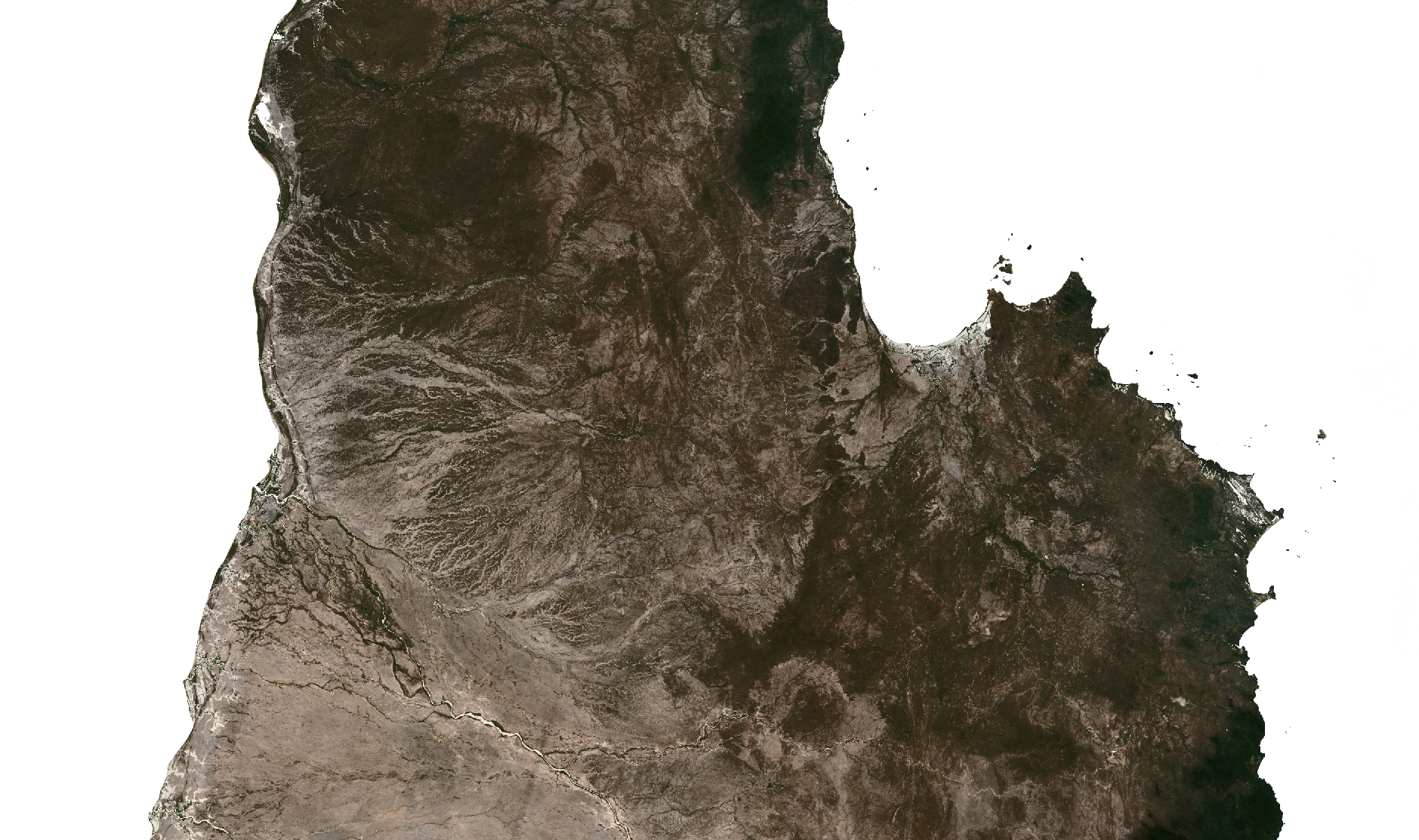
For this example, we return to the Queensland geomedian example data we used in the at the start of this HOWTO guide.
This example uses a simple red-green-blue visualisation as the base image, with transparency based on NDVI - pixels with NDVI over 0.5 are shown fully opaque, pixels with NDVI <= 0.0 are shown fully transparent with values between 0 and 0.5 shown partially transparent:
rgb_ndvi_transparency_cfg = {
    "components": {
        "red": {"red": 1.0},
        "green": {"green": 1.0},
        "blue": {"blue": 1.0},
        "alpha": {
            "function": "datacube_ows.band_utils.norm_diff",
            "kwargs": {
                "band1": "nir",
                "band2": "red",
                "scale_from": (0.0, 0.5),
                "scale_to": (0, 255)
            }
        },
    },
    "scale_range": (50, 3000),
}
In the next chapter we look at how to generate legends for datacube-ows styles.